
Blog 1: Challenges and future of robotic navigation in urban canyons
Date:
Robotics systems in urban canyons
I have been focusing on developing the reliable positioning solutions for the robotics systems for more than 7 years. To be specific, the positioning is one of the most fundermental components for the fully autonomous robotic systems, which tries to answer a question: where you are?
In the past decades, the positioning solution based on Simultaneously Localization And Mapping (SLAM) was extensively investigated. For example, the visual SLAM and LiDAR SLAM can provide very accuarte pose estimation estimation in a short period. However, these solutions are subjected to drift over time. The drift is even enhanced in highly urbanzied dynamic scenarios with following key challnenges:
- The inherent accumulated drift over time
- The impacts from the dynamic objects which can violate the assumption of the static features (usually the data association in SLAM assumes that the features are static)
On the contrary, the global navigation satellite systems (GNSS) can provide globally referenced and drift free positioning. Unfortunately, the GNSS signal is reflected by tall buildings in urban canyons, leading to the additional signal transmission delay. Typically, the positioning error can easily reach 10 meters even when the real-time kinematic technique is applied. In particular,the challenges lie in below aspects:
- The signal reflections from the surrounding buildings cause the additional signal transmission delay. In other words, the GNSS raw measurements, such as the pseudorange and Doppler measurements, are polluted. This could lead to non-line-of-sight (NLOS) and multipath effects.
- The signal blockage cause the poor satellite geometry as mainly the satellites with high elevation angles are received by the receiver in urban canyons.
One promising solution is to combine the advantage of the local positioning from the VSLAM or LiDAR SLAM, and the global positioning from the GNSS.
Mathematic formuation of positioning
Let’s consider the general form of the integration of the GNSS and local SLAM, it can be expressed as the below Maximum a posteriori (MAP) estimation problem:
\[P(x_t \mid z_{1: t}, u_{1: t}) =\sum_{m_{t-1}} P(z_t \mid x_t, u_{1: t}) \sum_{x_{t-1}} P(x_t \mid x_{t-1}) P(x_{t-1} \mid z_{t-1}, u_{1: t})\]where the $u_{t}$ denotes the control input such as the relative motion estimated by the visual or LiDAR SLAM. The $z_{t}$ denotes the absolute observation from the GNSS. Specifically, by applying the Gaussian nosie assumption, the factor graph optimization based formulation could be obtained as below:
\[({x_0,\ldots,x_t})^* =\arg \max _{x_0,\ldots,x_t} \sum_{j=0, \ldots, n} ({\lvert{\lvert h({z}_j, x_j)-z_j \rvert}\rvert}_{\Sigma_j}^{2} + \sum_{i=0, \ldots, m} {\lvert{\lvert h({z}_i, x_i, x_{i+1})-z_i \rvert}\rvert}_{\Sigma_i}^{2})\]where the $({x_0,\ldots,x_t})$ denotes all the states that is to be estimated at the current sliding window. The $\Sigma_j$ denotes the weighting associated with the global observation $z_j$. The $\Sigma_i$ denotes the weighting associated with the global observation $z_i$ which associates with the state $x_i$ and $x_{i+1}$. The factor graph optimization form could be solved iteratively and the optimal state could be gained based on the given measurements. However, the poor measurements from GNSS is included in the state estimation. As a result, the positioning accuracy could not be guaranteed. Is it possible that we explore the deep integration of the GNSS and local sensors, such as the LiDAR? How can we actively sense the surrounding environments and improve the quality of the GNSS measurements?
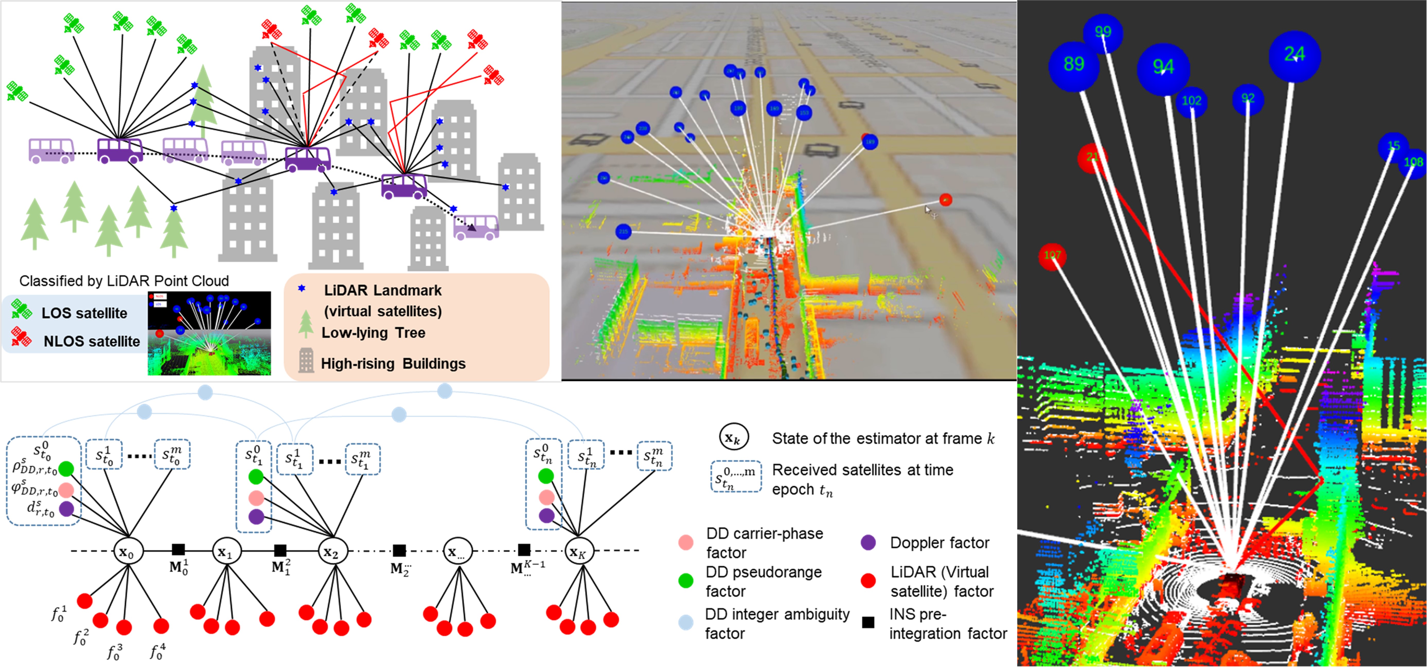
3D LiDAR aided GNSS positioning (3DLA GNSS)
In the past 4 years since 2018, we explore this possibility. Our idea is to employ the environmental description generated by 3D LiDAR to detect the GNSS NLOS receptions. One could use the 3D point clouds from the 3D LiDAR to detect the GNSS NLOS signal which will be further excluded from the GNSS positioning. However, this could lead to the poor satellite geometry. As a result, the GNSS positioning accuracy is still not guaranteed. Moreover, the multipath effect is not well handled which limits the performance of the GNSS positioning in urban canyons.
This finding can be very interesting which is different from our intuitive understanding. For example, the visual positioning can be improved once the outlier feature correspondance is removed. One of the reason is that the outlier visual correspondance is 100% outliers. Differently, the satellite measurements affected by the multipath effects involves the soft errors. For example, the error can range from 0.1 meters to 100 meters. When the GNSS signal is healthy, the observation model for the GNSS measurement, for example, the pseudorange measurement can be modelled as below:
\[\rho_{r,t}^{s}=r_{r}^{s}+c(\delta_{r,t}-\delta_{r,t}^{s})+I_{r,t}^{s}+T_{r,t}^{s}+\epsilon_{r,t}^{s}\]where the $\rho_{r,t}^{s}$ denotes the pseudorange measurement received from the satellite $s$ by the receiver $r$. The $r_{r}^{s}$ denotes the real range between the GNSS receiver and satellite. The $c$ denotes the speed of light. The $\delta_{r,t}$ and $\delta_{r,t}^{s}$ denotes the receiver and satellite clock bias. The $I_{r,t}^{s}$ and $T_{r,t}^{s}$ denotes the innospheric and tropospheric errors. The $\epsilon_{r,t}^{s}$ denotes the Gaussian noise associated with the pseudorange measurements. Let’s consider the polluted GNSS pseudorange measurements. The new observation model should be as below:
\[\rho_{r,t}^{s}=r_{r}^{s}+c(\delta_{r,t}-\delta_{r,t}^{s})+I_{r,t}^{s}+T_{r,t}^{s}+ b_{r,t}^{s}+\epsilon_{r,t}^{s}\]In particular, the $b_{r,t}^{s}$ denotes the bias caused by the signal reflection. How should we model the $b_{r,t}^{s}$?
Currently, the GNSS positioning is still challenging in urban canyons even using the 3DLA GNSS. There are still several problems to be investiagted:
- How to model the uncertainty of the multipath signal before its integration with other information?
- The GNSS NLOS exclusion can cause the poor satellite geometry, can we correct the GNSS NLOS error and re-use the GNSS NLOS signal? NLOS signal with multiple reflections is typical in urban canyons, how to model the GNSS NLOS routes with multiple reflections?
- Given the poor satellite geometry in urban canyons, the integer ambiguity of the carrier-phase is hard to be correctly resolved due to the poor satellite geometry. How to reliably resolve the ambiguity in urban canyons?
GNSS multipath re-modeling
Take the multipath signal as an example, the multiptath is almost impossible to be corrected as the multipath effect is the combination of the direct and reflected signals. One possible solution is to model the uncertainty of the multipath signals. Let’s consider the pseudorange measurements as an example:
\[({x_0,\ldots,x_t})^* =\arg \max _{x_0,\ldots,x_t} \sum_{j=0, \ldots, n} w_j {\lvert{\lvert h({z}_j, x_j,)-z_j \rvert}\rvert}_{2}^{2}\]where the $w_j$ denotes the weightings of the pseudorange measurements. If $w_j=0$, the pseudorange measurement is excluded. If $w_j<1$, this indicates that the measurments is de-weighted but is still used in the state estimation. In particular, the following is satisfied:
\[w_j={\Sigma_i}^{-1}\]This could maintain the satellite geometry and mitigate the impacts of the outliers simultaneously. However, the uncertainty estimation of the multipath is still a quite challenging problem.
In particular, the function to model the uncertainty of the GNSS multipath pseudorange measurement is mathematically derived as below [2]:
\[\sigma_{mp}=f(\alpha, d, \Delta \tau)\]where the $\sigma_{mp}$ denotes the potential error of the multipath signal. The $f(\alpha, d, \Delta \tau)$ is the envolope model which represents how the error is determined. The 𝑑 is the time spacing between early and late correlators directly from the GNSS receiver. The Δ𝜏 denotes the signal transmission delay caused by the signal reflection which is not available from the GNSS receiver. The $\alpha$ denotes the GNSS signal attenuation parameter, which indicates how the signal noise ratio decreases and is related to the material leading to the signal reflections. Unfortunately, the $\alpha$ is also a unknow variable.
References
- [1] Using latex to input equations in Overleaf Link.
- [2] L. Liu and M. G. Amin, “Tracking performance and average error analysis of GPS discriminators in multipath,” Signal Processing, vol. 89, no. 6, pp. 1224-1239, 2009/06/01/ 2009, doi