
Searching for Safety: Integrity-Aware Active Perception with Learned Search Policy for Autonomous Drone Navigation in Forest Environments
Date:
Searching for Safety: Integrity-Aware Active Perception with Learned Search Policy for Autonomous Drone Navigation in Forest Environments
Department of Aeronautical and Aviation Engineering, The Hong Kong Polytechnic University
Weisong Wen
Table of Contents
- Introduction and Motivation
- Problem Statement
- GNSS Measurement Model Under Forest Canopy
- Geometric Landmark Model: Tree Trunk Observations
- Tightly-Coupled Factor Graph Optimization
- ARAIM-Based Integrity Monitoring Framework
- Active Perception Formulation
- Reinforcement Learning Search Policy
- Reward Design and Training
- Experimental Validation
- Conclusions
- References
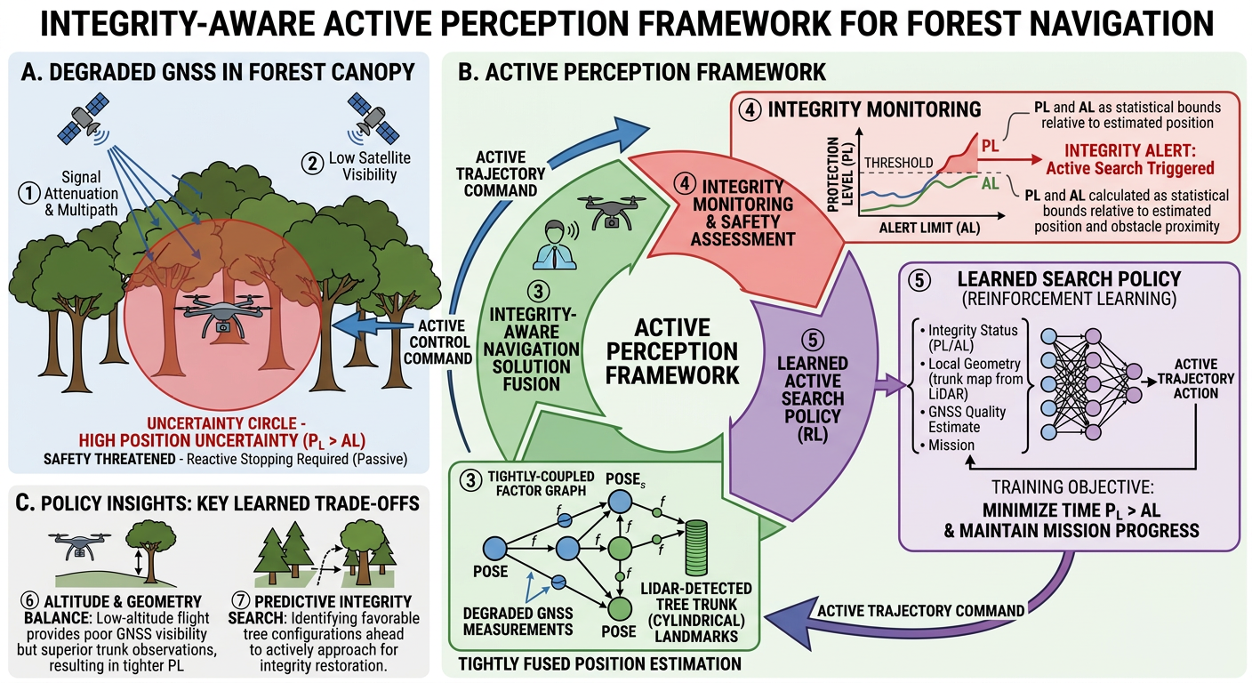
Figure 1. Overview of the Integrity-Aware Active Perception Framework for forest navigation. (A) Degraded GNSS in forest canopy with signal attenuation and multipath. (B) The active perception loop integrating tightly-coupled factor graph optimization, integrity monitoring, and a learned search policy. (C) Key learned trade-offs including altitude-geometry balance and predictive integrity search.
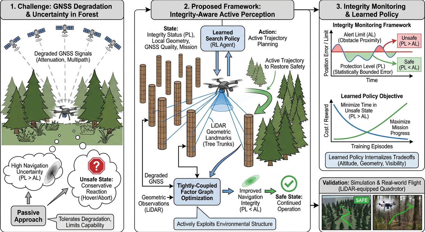
Figure 2. System concept showing the challenge of GNSS degradation in forest environments (left), the proposed integrity-aware active perception framework with tightly-coupled factor graph optimization and learned search policy (center), and the integrity monitoring and learned policy objective framework (right).
1. Introduction and Motivation
Autonomous drone operations in forest environments face a fundamental navigation safety challenge. Global Navigation Satellite System (GNSS) signals, while still partially available beneath the canopy, suffer significant degradation due to signal attenuation, multipath reflections, and reduced satellite visibility. This degradation inflates the uncertainty of the navigation solution unpredictably, creating periods where the drone cannot guarantee its position accuracy is sufficient for safe flight among densely distributed obstacles.
Conventional approaches address this problem reactively — slowing down, hovering, or aborting the mission when navigation uncertainty becomes excessive. Such conservative strategies severely limit operational capability in environments where reliable navigation is most critically needed.
This work proposes a novel framework that reframes the navigation safety problem as an integrity-aware active perception task. Rather than passively tolerating degraded GNSS integrity, the drone actively seeks trajectories that restore and maintain navigation safety by exploiting the geometric structure of the surrounding forest. Tree trunks, modeled as cylindrical primitives, serve as natural geometric landmarks whose spatial distribution provides observable constraints on the drone's position. By detecting and incorporating these geometric features into the navigation solution through a tightly-coupled factor graph optimization, the drone gains a complementary positioning source that compensates for GNSS degradation.
The central insight is that the informativeness of these geometric observations depends strongly on the spatial configuration of trees relative to the drone — analogous to how satellite geometry governs GNSS dilution of precision (DOP) — and the drone can actively influence this configuration through intelligent trajectory planning.
2. Problem Statement
We consider a quadrotor UAV navigating through a forest environment toward a goal location. The drone is equipped with:
- A GNSS receiver providing pseudorange measurements (degraded under canopy)
- An IMU providing high-rate inertial measurements
- A 3D LiDAR sensor capable of detecting and parameterizing nearby tree trunks
The drone's state at time $t$ is defined as:
$$\mathbf{x}_t = \begin{bmatrix} \mathbf{p}_t \\ \mathbf{v}_t \\ \mathbf{q}_t \\ \mathbf{b}_t^a \\ \mathbf{b}_t^g \\ \delta t_{\text{clk}} \\ \dot{\delta t}_{\text{clk}} \end{bmatrix} \in \mathbb{R}^3 \times \mathbb{R}^3 \times SO(3) \times \mathbb{R}^3 \times \mathbb{R}^3 \times \mathbb{R} \times \mathbb{R}$$where $\mathbf{p}_t$ is position, $\mathbf{v}_t$ is velocity, $\mathbf{q}_t$ is orientation (as a unit quaternion on $SO(3)$), $\mathbf{b}_t^a$ and $\mathbf{b}_t^g$ are accelerometer and gyroscope biases, and $\delta t_{\text{clk}}, \dot{\delta t}_{\text{clk}}$ are receiver clock bias and drift.
The navigation safety requirement is that the drone's true position error must remain bounded with high probability:
$$\Pr\left(\|\mathbf{p}_t - \hat{\mathbf{p}}_t\| \leq \text{PL}_t\right) \geq 1 - P_{\text{HMI}}$$where $\text{PL}_t$ is the protection level (a statistical bound on position error), $\hat{\mathbf{p}}_t$ is the estimated position, and $P_{\text{HMI}}$ is the tolerable probability of hazardous misleading information (typically $10^{-7}$ per epoch).
The safety condition is satisfied when:
$$\text{PL}_t < \text{AL}_t$$where $\text{AL}_t$ is the alert limit derived from the proximity to the nearest obstacles.
3. GNSS Measurement Model Under Forest Canopy
3.1 Pseudorange Observation Model
For the $j$-th visible satellite at time $t$, the pseudorange measurement is:
$$\rho_t^j = \|\mathbf{p}_t - \mathbf{p}_{\text{sat}}^j\| + c \cdot \delta t_{\text{clk}} + I_t^j + T_t^j + \epsilon_{\text{mp},t}^j + \eta_t^j$$where:
- $\mathbf{p}_{\text{sat}}^j$ is the known satellite position from broadcast ephemeris
- $c$ is the speed of light
- $I_t^j$ is the ionospheric delay (corrected by model)
- $T_t^j$ is the tropospheric delay (corrected by model)
- $\epsilon_{\text{mp},t}^j$ is the multipath error (dominant under canopy)
- $\eta_t^j \sim \mathcal{N}(0, \sigma_j^2)$ is receiver noise
After applying standard corrections, the pseudorange residual for factor graph integration becomes:
$$r_t^{\text{GNSS},j}(\mathbf{x}_t) = \tilde{\rho}_t^j - \|\mathbf{p}_t - \mathbf{p}_{\text{sat}}^j\| - c \cdot \delta t_{\text{clk}}$$3.2 Forest Canopy Degradation Model
Under forest canopy, the effective pseudorange variance is inflated as a function of canopy density $\kappa$ and satellite elevation $\theta^j$:
$$\sigma_{\text{eff},j}^2 = \sigma_0^2 + \frac{\sigma_{\text{mp}}^2}{\sin^2(\theta^j)} + \sigma_{\text{canopy}}^2(\kappa, \theta^j)$$where the canopy attenuation term follows a Beer-Lambert-inspired model:
$$\sigma_{\text{canopy}}^2(\kappa, \theta^j) = \sigma_c^2 \cdot \exp\left(\frac{\alpha \cdot \kappa}{\sin(\theta^j)}\right)$$with $\alpha$ being the attenuation coefficient dependent on foliage type and density. The number of visible satellites $N_{\text{vis}}$ also decreases with canopy density, further degrading the geometric dilution of precision (GDOP).
3.3 GNSS Geometry and DOP
The satellite geometry matrix for $N$ visible satellites is:
$$\mathbf{G} = \begin{bmatrix} -\mathbf{e}_1^\top & 1 \\ -\mathbf{e}_2^\top & 1 \\ \vdots & \vdots \\ -\mathbf{e}_N^\top & 1 \end{bmatrix}$$where $\mathbf{e}_j = \frac{\mathbf{p}_{\text{sat}}^j - \hat{\mathbf{p}}_t}{\|\mathbf{p}_{\text{sat}}^j - \hat{\mathbf{p}}_t\|}$ is the unit line-of-sight vector. The position DOP is:
$$\text{PDOP} = \sqrt{\text{tr}\left([\mathbf{H}]_{1:3,1:3}\right)}, \quad \mathbf{H} = (\mathbf{G}^\top \mathbf{W} \mathbf{G})^{-1}$$where $\mathbf{W} = \text{diag}(\sigma_{\text{eff},1}^{-2}, \ldots, \sigma_{\text{eff},N}^{-2})$ is the weighting matrix. Under canopy, both reduced $N_{\text{vis}}$ and inflated $\sigma_{\text{eff},j}^2$ cause PDOP to increase dramatically.
4. Geometric Landmark Model: Tree Trunk Observations
4.1 Cylindrical Primitive Parameterization
Each tree trunk $k$ detected by LiDAR is modeled as a vertical cylinder parameterized by its center position in the horizontal plane and radius:
$$\mathcal{T}_k = \left(\mathbf{c}_k, r_k\right), \quad \mathbf{c}_k = \begin{bmatrix} c_{k,x} \\ c_{k,y} \end{bmatrix} \in \mathbb{R}^2, \quad r_k \in \mathbb{R}^+$$Given a horizontal LiDAR scan slice, points belonging to trunk $k$ are segmented via Euclidean clustering and fit to a circle using least-squares:
$$\hat{\mathbf{c}}_k, \hat{r}_k = \underset{\mathbf{c}, r}{\arg\min} \sum_{i=1}^{M_k} \left(\|\mathbf{p}_{\text{lidar},i} - \mathbf{c}\| - r\right)^2$$where $M_k$ is the number of LiDAR points associated with trunk $k$ and $\mathbf{p}_{\text{lidar},i}$ are the point positions in the sensor frame.
4.2 Trunk Observation Factor
The observation of trunk $k$ from drone pose $\mathbf{x}_t$ produces a range-bearing measurement in the body frame. Transforming to the global frame, the geometric residual is:
$$\mathbf{r}_t^{\text{trunk},k}(\mathbf{x}_t, \mathbf{c}_k) = \mathbf{R}(\mathbf{q}_t)^\top \left(\mathbf{c}_k^{3D} - \mathbf{p}_t\right) - \tilde{\mathbf{z}}_t^k$$where $\mathbf{R}(\mathbf{q}_t)$ is the rotation matrix from the drone's orientation, $\mathbf{c}_k^{3D} = [c_{k,x}, c_{k,y}, z_{\text{obs}}]^\top$ is the 3D observation point on the trunk, and $\tilde{\mathbf{z}}_t^k$ is the LiDAR measurement in the body frame.
The measurement covariance for trunk observations is:
$$\boldsymbol{\Sigma}_{\text{trunk},k} = \text{diag}\left(\sigma_{\text{range}}^2, \sigma_{\text{bearing}}^2, \sigma_z^2\right)$$where $\sigma_{\text{range}}$ depends on LiDAR specifications and the number of points $M_k$, and $\sigma_{\text{bearing}}$ depends on angular resolution and trunk curvature.
4.3 Geometric Dilution of Precision from Trees (TDOP)
Analogous to satellite GDOP, we define a Tree Dilution of Precision (TDOP) that characterizes the geometric strength of trunk observations. For $K$ observed trunks with unit direction vectors $\mathbf{u}_k = \frac{\mathbf{c}_k - \hat{\mathbf{p}}_t^{xy}}{\|\mathbf{c}_k - \hat{\mathbf{p}}_t^{xy}\|}$, form the geometry matrix:
$$\mathbf{G}_{\text{tree}} = \begin{bmatrix} \mathbf{u}_1^\top \\ \mathbf{u}_2^\top \\ \vdots \\ \mathbf{u}_K^\top \end{bmatrix} \in \mathbb{R}^{K \times 2}$$The horizontal TDOP is:
$$\text{TDOP} = \sqrt{\text{tr}\left(\left(\mathbf{G}_{\text{tree}}^\top \mathbf{W}_{\text{tree}} \mathbf{G}_{\text{tree}}\right)^{-1}\right)}$$where $\mathbf{W}_{\text{tree}} = \text{diag}(\sigma_{\text{trunk},1}^{-2}, \ldots, \sigma_{\text{trunk},K}^{-2})$. A lower TDOP indicates stronger geometric constraints. Critically, TDOP depends on the angular spread of observed trunks — trunks clustered in one direction provide poor geometry, while trunks distributed around the drone provide strong constraints.
5. Tightly-Coupled Factor Graph Optimization
5.1 Factor Graph Formulation
The navigation solution is estimated by maximizing the posterior probability over a sliding window of states $\mathcal{X} = \{\mathbf{x}_{t-W}, \ldots, \mathbf{x}_t\}$ and landmark positions $\mathcal{L} = \{\mathbf{c}_1, \ldots, \mathbf{c}_K\}$:
$$\hat{\mathcal{X}}, \hat{\mathcal{L}} = \underset{\mathcal{X}, \mathcal{L}}{\arg\max}\ p(\mathcal{X}, \mathcal{L} \mid \mathcal{Z})$$where $\mathcal{Z}$ denotes all measurements. Under Gaussian noise assumptions, this is equivalent to the nonlinear least-squares problem:
$$\hat{\mathcal{X}}, \hat{\mathcal{L}} = \underset{\mathcal{X}, \mathcal{L}}{\arg\min}\ \underbrace{\sum_{\tau} \|\mathbf{r}^{\text{IMU}}_\tau(\mathbf{x}_\tau, \mathbf{x}_{\tau+1})\|^2_{\boldsymbol{\Sigma}_{\text{IMU},\tau}}}_{\text{IMU preintegration factors}} + \underbrace{\sum_{\tau} \sum_{j \in \mathcal{V}_\tau} \|\mathbf{r}^{\text{GNSS},j}_\tau(\mathbf{x}_\tau)\|^2_{\sigma_{\text{eff},j}^2}}_{\text{GNSS pseudorange factors}} + \underbrace{\sum_{\tau} \sum_{k \in \mathcal{O}_\tau} \|\mathbf{r}^{\text{trunk},k}_\tau(\mathbf{x}_\tau, \mathbf{c}_k)\|^2_{\boldsymbol{\Sigma}_{\text{trunk},k}}}_{\text{Tree trunk observation factors}}$$where $\|\mathbf{r}\|^2_{\boldsymbol{\Sigma}} = \mathbf{r}^\top \boldsymbol{\Sigma}^{-1} \mathbf{r}$ denotes the Mahalanobis norm, $\mathcal{V}_\tau$ is the set of visible satellites at time $\tau$, and $\mathcal{O}_\tau$ is the set of observed trunks.
5.2 IMU Preintegration Factor
Between consecutive keyframes $\mathbf{x}_\tau$ and $\mathbf{x}_{\tau+1}$, IMU measurements are preintegrated following the formulation of Forster et al. [1]. The preintegrated measurements are:
$$\Delta \tilde{\mathbf{p}}_{\tau,\tau+1} = \sum_{i=\tau}^{\tau+1} \left[\Delta \tilde{\mathbf{v}}_{\tau,i} \cdot \Delta t + \frac{1}{2} \Delta \tilde{\mathbf{R}}_{\tau,i} (\tilde{\mathbf{a}}_i - \mathbf{b}_\tau^a) \Delta t^2\right]$$ $$\Delta \tilde{\mathbf{v}}_{\tau,\tau+1} = \sum_{i=\tau}^{\tau+1} \Delta \tilde{\mathbf{R}}_{\tau,i} (\tilde{\mathbf{a}}_i - \mathbf{b}_\tau^a) \Delta t$$ $$\Delta \tilde{\mathbf{R}}_{\tau,\tau+1} = \prod_{i=\tau}^{\tau+1} \text{Exp}\left((\tilde{\boldsymbol{\omega}}_i - \mathbf{b}_\tau^g) \Delta t\right)$$The IMU residual vector encapsulates position, velocity, and rotation errors:
$$\mathbf{r}^{\text{IMU}}_\tau = \begin{bmatrix} \mathbf{R}_\tau^\top(\mathbf{p}_{\tau+1} - \mathbf{p}_\tau - \mathbf{v}_\tau \Delta T - \frac{1}{2}\mathbf{g}\Delta T^2) - \Delta \tilde{\mathbf{p}}_{\tau,\tau+1} \\ \mathbf{R}_\tau^\top(\mathbf{v}_{\tau+1} - \mathbf{v}_\tau - \mathbf{g}\Delta T) - \Delta \tilde{\mathbf{v}}_{\tau,\tau+1} \\ \text{Log}\left(\Delta \tilde{\mathbf{R}}_{\tau,\tau+1}^\top \mathbf{R}_\tau^\top \mathbf{R}_{\tau+1}\right) \end{bmatrix}$$5.3 Solution via Gauss-Newton / iSAM2
The factor graph is solved incrementally using iSAM2 [2]. At each step, the linearized system takes the form:
$$\mathbf{J}^\top \boldsymbol{\Sigma}^{-1} \mathbf{J} \cdot \delta \mathbf{x}^* = -\mathbf{J}^\top \boldsymbol{\Sigma}^{-1} \mathbf{r}(\hat{\mathbf{x}})$$where $\mathbf{J}$ is the stacked Jacobian of all residuals. The posterior covariance of the current state estimate is extracted from the Bayes tree:
$$\boldsymbol{\Sigma}_{\hat{\mathbf{x}}_t} = \left(\mathbf{J}_t^\top \boldsymbol{\Sigma}^{-1} \mathbf{J}_t\right)^{-1}$$The position covariance block $\boldsymbol{\Sigma}_{\hat{\mathbf{p}}_t} \in \mathbb{R}^{3\times 3}$ is the key input to the integrity monitoring module.
6. ARAIM-Based Integrity Monitoring Framework
We adopt an integrity monitoring framework grounded in the Advanced Receiver Autonomous Integrity Monitoring (ARAIM) methodology developed for multi-constellation GNSS aviation applications [3, 8]. The ARAIM framework provides a rigorous, probabilistically certified approach to bounding position errors in the presence of potential measurement faults. We extend this framework from the standard weighted least-squares (WLS) context to the tightly-coupled factor graph optimization (FGO) setting and further incorporate geometric landmark observations.
6.1 Integrity Risk Definitions and Requirements
Navigation integrity is defined through the following probabilistic quantities [3, 11]:
- Hazardous Misleading Information (HMI): An HMI event occurs when the true position error exceeds the alert limit without a timely alert being issued. The probability of HMI must satisfy: $$P_{\text{HMI}} = \Pr\left(\|\mathbf{p}_t - \hat{\mathbf{p}}_t\|_q > \text{AL}_q \ \cap \ \text{no alert issued}\right) \leq P_{\text{HMI,req}}$$ where $\|\cdot\|_q$ denotes the position error projected onto direction $q$ (horizontal or vertical), and $P_{\text{HMI,req}}$ is the required integrity risk (typically $10^{-7}$ per epoch for aviation, adapted here for UAV operations).
- Protection Level (PL): A real-time, overbounding statistic computed by the navigation system such that: $$\Pr\left(\|\mathbf{p}_t - \hat{\mathbf{p}}_t\|_q > \text{PL}_q\right) \leq P_{\text{HMI,req}}$$ The system is declared available (safe) when $\text{PL}_q < \text{AL}_q$.
- Continuity Risk: The probability of false alert: $$P_{\text{FA}} = \Pr\left(\text{alert issued} \ | \ \text{no fault present}\right) \leq P_{\text{FA,req}}$$
6.2 ARAIM Threat Model and Fault Hypothesis
The ARAIM threat model considers a discrete set of fault hypotheses $\mathcal{H} = \{H_0, H_1, \ldots, H_{N_f}\}$:
| Hypothesis | Description | Prior Probability |
|---|---|---|
| $H_0$ | Fault-free: all measurements nominal | $P_0 = 1 - \sum_{i} P_{sat,i} - \sum_{c} P_{const,c}$ |
| $H_i\ (i=1,\ldots,N)$ | Single satellite fault: satellite $i$ has an undetected bias | $P_{sat,i}$ (from ISM, typ. $10^{-5}$ per satellite) |
| $H_c\ (c=1,\ldots,C)$ | Constellation-wide fault: all satellites from constellation $c$ biased | $P_{const,c}$ (from ISM, typ. $10^{-4}$ per constellation) |
| $H_k^{\text{trunk}}\ (k=1,\ldots,K)$ | Trunk landmark fault: tree $k$ misassociated or incorrectly parameterized | $P_{trunk,k}$ (environment-dependent) |
Here ISM denotes the Integrity Support Message providing the a priori fault probabilities $P_{sat,i}$ and $P_{const,c}$ as broadcast parameters. For tree trunk observations, we define analogous prior fault probabilities $P_{trunk,k}$ based on detection confidence from the LiDAR segmentation pipeline.
The total number of fault hypotheses is:
$$N_f = N + C + K$$where $N$ is the number of satellites, $C$ is the number of constellations, and $K$ is the number of observed tree trunks.
6.3 Integrity Risk Allocation
The total integrity risk budget $P_{\text{HMI,req}}$ is decomposed across all fault hypotheses using the law of total probability [3]:
$$P_{\text{HMI}} = \underbrace{P_{\text{HMI}|H_0} \cdot P_0}_{\text{fault-free risk}} + \underbrace{\sum_{i=1}^{N} P_{\text{HMI}|H_i} \cdot P_{sat,i}}_{\text{single satellite fault risk}} + \underbrace{\sum_{c=1}^{C} P_{\text{HMI}|H_c} \cdot P_{const,c}}_{\text{constellation fault risk}} + \underbrace{\sum_{k=1}^{K} P_{\text{HMI}|H_k^{\text{trunk}}} \cdot P_{trunk,k}}_{\text{trunk landmark fault risk}}$$To satisfy $P_{\text{HMI}} \leq P_{\text{HMI,req}}$, we allocate the integrity budget as:
$$P_{\text{HMI,req}} = P_{\text{HMI,alloc},0} + \sum_{i=1}^{N} P_{\text{HMI,alloc},i} + \sum_{c=1}^{C} P_{\text{HMI,alloc},c} + \sum_{k=1}^{K} P_{\text{HMI,alloc},k}^{\text{trunk}}$$A common allocation strategy assigns equal budgets to the fault-free and faulted modes:
$$P_{\text{HMI,alloc},0} = \frac{P_{\text{HMI,req}}}{2}, \qquad P_{\text{HMI,alloc},i} = \frac{P_{\text{HMI,req}}}{2(N + C + K)} \quad \forall\ i$$Similarly, the continuity (false alert) budget is allocated:
$$P_{\text{FA,req}} = \sum_{k=1}^{N_f} P_{\text{FA,alloc},k}$$6.4 Solution Separation Method
The ARAIM protection level is computed via the solution separation technique [3, 12]. For each fault hypothesis $H_k$, a subset solution is computed by excluding or down-weighting the suspected faulty measurements.
6.4.1 Full and Subset Solutions in the WLS Context
In the linearized WLS framework, the full (all-in-view) position solution at epoch $t$ is:
$$\hat{\mathbf{x}}^{(0)} = \left(\mathbf{G}^\top \mathbf{W}_0 \mathbf{G}\right)^{-1} \mathbf{G}^\top \mathbf{W}_0 \mathbf{y}$$where $\mathbf{G} \in \mathbb{R}^{M \times n}$ is the combined geometry matrix (rows from both GNSS satellites and tree trunk observations), $\mathbf{y} \in \mathbb{R}^M$ is the measurement residual vector, $\mathbf{W}_0 = \text{diag}(\sigma_1^{-2}, \ldots, \sigma_M^{-2})$ is the nominal weighting matrix, and $n$ is the state dimension.
For fault hypothesis $H_k$, the subset solution uses a modified weight matrix $\mathbf{W}_k$ that excludes the suspected faulty measurements:
$$\hat{\mathbf{x}}^{(k)} = \left(\mathbf{G}^\top \mathbf{W}_k \mathbf{G}\right)^{-1} \mathbf{G}^\top \mathbf{W}_k \mathbf{y}$$where $\mathbf{W}_k$ is identical to $\mathbf{W}_0$ except that the weight(s) corresponding to fault mode $k$ are set to zero:
$$[\mathbf{W}_k]_{jj} = \begin{cases} 0 & \text{if measurement } j \text{ is suspected under } H_k \\ [\mathbf{W}_0]_{jj} & \text{otherwise} \end{cases}$$Define the projection (solution) matrices:
$$\mathbf{S}_0 = \left(\mathbf{G}^\top \mathbf{W}_0 \mathbf{G}\right)^{-1} \mathbf{G}^\top \mathbf{W}_0, \qquad \mathbf{S}_k = \left(\mathbf{G}^\top \mathbf{W}_k \mathbf{G}\right)^{-1} \mathbf{G}^\top \mathbf{W}_k$$6.4.2 Extension to Factor Graph Optimization
In our FGO framework, the solutions are obtained from the linearized factor graph rather than single-epoch WLS. The full solution covariance is extracted from the information matrix (Hessian) of the factor graph [2, 6]:
$$\boldsymbol{\Lambda}^{(0)} = \sum_{\tau} \mathbf{J}_{\text{IMU},\tau}^\top \boldsymbol{\Sigma}_{\text{IMU},\tau}^{-1} \mathbf{J}_{\text{IMU},\tau} + \sum_{\tau}\sum_{j \in \mathcal{V}_\tau} \frac{1}{\sigma_{\text{eff},j}^2} \mathbf{J}_{\text{GNSS},j}^\top \mathbf{J}_{\text{GNSS},j} + \sum_{\tau}\sum_{k \in \mathcal{O}_\tau} \mathbf{J}_{\text{trunk},k}^\top \boldsymbol{\Sigma}_{\text{trunk},k}^{-1} \mathbf{J}_{\text{trunk},k}$$where $\mathbf{J}_{\text{IMU},\tau}$, $\mathbf{J}_{\text{GNSS},j}$, and $\mathbf{J}_{\text{trunk},k}$ are the Jacobians of the respective residuals evaluated at the current estimate. The full solution covariance for the current position is the marginal:
$$\boldsymbol{\Sigma}^{(0)} = \left[\left(\boldsymbol{\Lambda}^{(0)}\right)^{-1}\right]_{\mathbf{p}_t, \mathbf{p}_t}$$For subset solution $k$ (fault hypothesis $H_k$), the information matrix is recomputed with the suspected faulty measurement(s) removed:
$$\boldsymbol{\Lambda}^{(k)} = \boldsymbol{\Lambda}^{(0)} - \underbrace{\mathbf{J}_k^\top \boldsymbol{\Sigma}_k^{-1} \mathbf{J}_k}_{\text{information from excluded measurement(s)}}$$ $$\boldsymbol{\Sigma}^{(k)} = \left[\left(\boldsymbol{\Lambda}^{(k)}\right)^{-1}\right]_{\mathbf{p}_t, \mathbf{p}_t}$$The solution separation vector between the full and subset solutions is:
$$\mathbf{d}_k = \hat{\mathbf{p}}_t^{(0)} - \hat{\mathbf{p}}_t^{(k)}$$6.4.3 Solution Separation Statistics
The covariance of the solution separation is derived from the difference of the two projection operators [3]:
$$\boldsymbol{\Sigma}_{ss,k} = \boldsymbol{\Sigma}^{(0)} + \boldsymbol{\Sigma}^{(k)} - \boldsymbol{\Sigma}^{(0)} \left(\boldsymbol{\Lambda}^{(0)} - \boldsymbol{\Lambda}^{(k)}\right) \boldsymbol{\Sigma}^{(k)} - \boldsymbol{\Sigma}^{(k)} \left(\boldsymbol{\Lambda}^{(0)} - \boldsymbol{\Lambda}^{(k)}\right) \boldsymbol{\Sigma}^{(0)}$$For the standard WLS case, this simplifies to:
$$\boldsymbol{\Sigma}_{ss,k} = (\mathbf{S}_0 - \mathbf{S}_k) \mathbf{C}_y (\mathbf{S}_0 - \mathbf{S}_k)^\top$$where $\mathbf{C}_y$ is the measurement noise covariance. The solution separation standard deviation projected onto direction $q$ (horizontal East, horizontal North, or vertical) is:
$$\sigma_{ss,q,k} = \sqrt{\mathbf{e}_q^\top \boldsymbol{\Sigma}_{ss,k} \mathbf{e}_q}$$where $\mathbf{e}_q$ is the unit projection vector for direction $q$.
6.5 Fault Detection Threshold
For each fault hypothesis $H_k$ and projection direction $q$, the detection threshold is set to control the false alert rate:
$$T_{q,k} = K_{\text{fa},k} \cdot \sigma_{ss,q,k}$$where $K_{\text{fa},k}$ is the false alert multiplier satisfying:
$$Q(K_{\text{fa},k}) = \frac{P_{\text{FA,alloc},k}}{2}$$and $Q(\cdot)$ is the tail probability of the standard normal distribution:
$$Q(x) = \frac{1}{\sqrt{2\pi}} \int_x^{\infty} e^{-u^2/2}\, du$$A fault is detected for hypothesis $H_k$ when the solution separation exceeds the threshold:
$$|d_{q,k}| = |\mathbf{e}_q^\top \mathbf{d}_k| > T_{q,k}$$6.6 Protection Level Computation via ARAIM
The protection level is the maximum over the fault-free and all faulted contributions, ensuring the integrity risk bound holds under every hypothesis [3]:
6.6.1 Fault-Free Protection Level
Under $H_0$ (no fault), the position error is Gaussian with covariance $\boldsymbol{\Sigma}^{(0)}$. The fault-free protection level in direction $q$ is:
$$\text{PL}_{q,0} = K_{ff,q} \cdot \sigma_{q,0}$$where $\sigma_{q,0} = \sqrt{\mathbf{e}_q^\top \boldsymbol{\Sigma}^{(0)} \mathbf{e}_q}$ is the standard deviation of the position error from the full solution in direction $q$, and $K_{ff,q}$ is the multiplier satisfying:
$$Q(K_{ff,q}) = \frac{P_{\text{HMI,alloc},0}}{2}$$For a typical allocation of $P_{\text{HMI,alloc},0} = 5 \times 10^{-8}$ (half the total budget):
$$K_{ff,q} = Q^{-1}\left(2.5 \times 10^{-8}\right) \approx 5.42$$6.6.2 Faulted Protection Level (Solution Separation Bound)
Under fault hypothesis $H_k$, the position error may contain an undetected bias. The protection level must account for (a) the maximum undetected bias that can pass the detection test and (b) the noise in the subset solution. The faulted protection level in direction $q$ is [3]:
$$\text{PL}_{q,k} = \underbrace{|d_{q,k}|}_{\text{observed separation}} + \underbrace{K_{\text{fa},k} \cdot \sigma_{ss,q,k}}_{\text{detection threshold}} + \underbrace{K_{\text{md},k} \cdot \sigma_{q,k}}_{\text{missed detection margin}}$$where:
- $|d_{q,k}|$ is the current observed solution separation magnitude
- $K_{\text{fa},k} \cdot \sigma_{ss,q,k} = T_{q,k}$ is the detection threshold (any bias below this is undetectable)
- $\sigma_{q,k} = \sqrt{\mathbf{e}_q^\top \boldsymbol{\Sigma}^{(k)} \mathbf{e}_q}$ is the position std from the subset solution
- $K_{\text{md},k}$ is the missed detection multiplier satisfying: $$Q(K_{\text{md},k}) = \frac{P_{\text{HMI,alloc},k}}{P_{\text{prior},k}}$$ with $P_{\text{prior},k}$ being the a priori fault probability ($P_{sat,i}$, $P_{const,c}$, or $P_{trunk,k}$)
Remark: When no fault is present (i.e., $|d_{q,k}| \ll T_{q,k}$), the faulted PL reduces to approximately $T_{q,k} + K_{\text{md},k} \cdot \sigma_{q,k}$. When a fault is detected ($|d_{q,k}| > T_{q,k}$), the faulty measurement is excluded and the solution is recomputed.
6.6.3 Overall Protection Level
The ARAIM protection level in direction $q$ is the maximum across all hypotheses:
$$\boxed{\text{PL}_q = \max\left(\text{PL}_{q,0},\ \max_{k=1,\ldots,N_f} \text{PL}_{q,k}\right)}$$The horizontal and vertical protection levels are:
$$\text{HPL} = \max\left(\text{PL}_{E},\ \text{PL}_{N}\right) \quad \text{or equivalently} \quad \text{HPL} = \sqrt{\text{PL}_{E}^2 + \text{PL}_{N}^2}$$ $$\text{VPL} = \text{PL}_{U}$$where subscripts $E$, $N$, $U$ denote East, North, and Up directions respectively. For 3D navigation safety in the forest environment:
$$\text{PL}_t = \max\left(\text{HPL}_t,\ \text{VPL}_t\right)$$6.7 Sensitivity Analysis: How Tree Observations Reduce PL
The key insight connecting integrity monitoring to active perception is how tree trunk observations reduce the protection level. Adding $K$ trunk observations to the factor graph modifies the information matrix:
$$\boldsymbol{\Lambda}^{(0)}_{\text{with trees}} = \boldsymbol{\Lambda}^{(0)}_{\text{GNSS+IMU}} + \underbrace{\sum_{k=1}^{K} \mathbf{J}_{\text{trunk},k}^\top \boldsymbol{\Sigma}_{\text{trunk},k}^{-1} \mathbf{J}_{\text{trunk},k}}_{\Delta \boldsymbol{\Lambda}_{\text{tree}}}$$This additional information reduces the position covariance:
$$\boldsymbol{\Sigma}^{(0)}_{\text{with trees}} \preceq \boldsymbol{\Sigma}^{(0)}_{\text{GNSS+IMU}}$$(in the positive semi-definite ordering), which directly reduces $\sigma_{q,0}$ and hence $\text{PL}_{q,0}$. Furthermore, the trunk observations provide independent fault detection capability — if a GNSS satellite is faulted, the trunk-based subset solution $\hat{\mathbf{p}}^{(k)}$ (excluding satellite $k$) is strengthened by the trunk information, reducing $\sigma_{q,k}$ and hence $\text{PL}_{q,k}$. This dual benefit (improved fault-free accuracy and improved fault detection/exclusion) is central to the active perception strategy.
6.8 Alert Limit from Obstacle Proximity
The alert limit $\text{AL}$ defines the maximum tolerable position error given the current obstacle environment. Unlike aviation where AL is a fixed operational parameter (e.g., 40 m for en-route, 0.3 m for CAT III landing), for drone navigation in forests the AL is dynamic and derived from the local obstacle geometry:
$$\text{HAL}_t = \gamma_H \cdot \min_{k \in \mathcal{N}_t} \left(\|\hat{\mathbf{p}}_t^{xy} - \mathbf{c}_k\| - r_k - r_{\text{drone}}\right)$$ $$\text{VAL}_t = \gamma_V \cdot \min\left(h_t - h_{\text{min}},\ h_{\text{canopy}} - h_t\right)$$where $\gamma_H, \gamma_V \in (0,1)$ are safety factors (typically 0.5), $\mathcal{N}_t$ is the set of nearby obstacles, $r_k$ is the trunk radius, $r_{\text{drone}}$ is the drone collision radius, $h_{\text{min}}$ is the minimum safe altitude above ground, and $h_{\text{canopy}}$ is the canopy height. The combined alert limit is:
$$\text{AL}_t = \min\left(\text{HAL}_t,\ \text{VAL}_t\right)$$6.9 Integrity State and Active Search Trigger
The ARAIM integrity assessment yields the following navigation states:
$$\mathcal{I}_t = \begin{cases} \textbf{SAFE} & \text{if } \text{PL}_t < \text{AL}_t \text{ and no fault detected} \\[4pt] \textbf{SAFE (excluded)} & \text{if fault detected, excluded, and } \text{PL}_t^{\text{excl}} < \text{AL}_t \\[4pt] \textbf{UNSAFE} & \text{if } \text{PL}_t \geq \text{AL}_t \text{ (integrity unavailable)} \end{cases}$$The integrity margin quantifies the safety budget:
$$\text{IM}_t = \text{AL}_t - \text{PL}_t$$The active search policy is triggered when:
$$\text{IM}_t \leq \text{IM}_{\text{threshold}}$$where $\text{IM}_{\text{threshold}} > 0$ is a configurable threshold that proactively activates the search before the integrity margin reaches zero, providing a buffer for the drone to find favorable geometry before safety is compromised. When $\text{IM}_t \leq 0$, the system is in a critical unsafe state and the search policy operates with maximum urgency.
6.10 Summary of ARAIM PL Computation Algorithm
The complete ARAIM protection level computation at each epoch proceeds as follows:
- Input: Measurement set $\mathcal{Z}_t$, geometry matrix $\mathbf{G}$, measurement covariances, ISM parameters $(P_{sat,i}, P_{const,c})$, trunk fault probabilities $P_{trunk,k}$, integrity/continuity budgets $(P_{\text{HMI,req}}, P_{\text{FA,req}})$
- Allocate integrity and continuity budgets across all $N_f + 1$ hypotheses
- Compute full solution $\hat{\mathbf{p}}^{(0)}$ and covariance $\boldsymbol{\Sigma}^{(0)}$ from FGO
- For each fault hypothesis $k = 1, \ldots, N_f$:
- Compute subset solution $\hat{\mathbf{p}}^{(k)}$ and covariance $\boldsymbol{\Sigma}^{(k)}$
- Compute solution separation $\mathbf{d}_k$ and its std $\sigma_{ss,q,k}$
- Compute detection threshold $T_{q,k}$
- Compute missed detection multiplier $K_{\text{md},k}$
- Compute faulted PL: $\text{PL}_{q,k} = |d_{q,k}| + T_{q,k} + K_{\text{md},k} \cdot \sigma_{q,k}$
- If $|d_{q,k}| > T_{q,k}$: flag measurement(s) for exclusion
- Compute fault-free PL: $\text{PL}_{q,0} = K_{ff,q} \cdot \sigma_{q,0}$
- Output: $\text{PL}_q = \max(\text{PL}_{q,0}, \max_k \text{PL}_{q,k})$; fault detection flags; integrity state $\mathcal{I}_t$
7. Active Perception Formulation
7.1 Information-Theoretic Objective
The goal of active perception is to plan trajectories that maximize the information gained about the drone's position. Given a candidate trajectory $\boldsymbol{\tau} = \{\mathbf{x}_{t+1}, \ldots, \mathbf{x}_{t+H}\}$ over planning horizon $H$, the expected information gain is:
$$\mathcal{I}(\boldsymbol{\tau}) = \mathbb{E}\left[\log \frac{|\boldsymbol{\Sigma}_{\hat{\mathbf{p}}_t}|}{|\boldsymbol{\Sigma}_{\hat{\mathbf{p}}_{t+H}}(\boldsymbol{\tau})|}\right]$$where $|\cdot|$ denotes the determinant and $\boldsymbol{\Sigma}_{\hat{\mathbf{p}}_{t+H}}(\boldsymbol{\tau})$ is the predicted position covariance at the end of the trajectory. This is equivalent to maximizing the mutual information between the trajectory and the position estimate.
7.2 Predicted Covariance and ARAIM PL Propagation
For a candidate trajectory, the predicted posterior covariance is computed by propagating through the factor graph structure. At each future step $\tau$ along the trajectory, the predicted information matrix is:
$$\boldsymbol{\Lambda}_{\tau+1}^{\text{pred}} = \boldsymbol{\Lambda}_{\tau|\text{IMU}} + \underbrace{\sum_{j \in \hat{\mathcal{V}}_{\tau+1}} \frac{1}{\sigma_{\text{eff},j}^2} \mathbf{J}_{\text{GNSS},j}^\top \mathbf{J}_{\text{GNSS},j}}_{\text{predicted GNSS information}} + \underbrace{\sum_{k \in \hat{\mathcal{O}}_{\tau+1}} \mathbf{J}_{\text{trunk},k}^\top \boldsymbol{\Sigma}_{\text{trunk},k}^{-1} \mathbf{J}_{\text{trunk},k}}_{\text{predicted trunk information}}$$where $\hat{\mathcal{V}}_{\tau+1}$ and $\hat{\mathcal{O}}_{\tau+1}$ are the predicted sets of visible satellites and observable trunks from the candidate position, $\boldsymbol{\Lambda}_{\tau|\text{IMU}}$ is the IMU-propagated information matrix, and $\mathbf{J}_{\text{trunk},k}$ is the Jacobian of the trunk observation. The predicted position covariance is $\boldsymbol{\Sigma}_{\tau+1}^{\text{pred}} = [(\boldsymbol{\Lambda}_{\tau+1}^{\text{pred}})^{-1}]_{\mathbf{p},\mathbf{p}}$.
Crucially, the predicted ARAIM protection level $\text{PL}_\tau^{\text{pred}}(\boldsymbol{\tau})$ at each future waypoint is computed using the full solution separation procedure from Section 6, with predicted measurements and geometry. This allows the planner to evaluate not just covariance reduction, but the actual integrity metric that governs safety.
7.3 Integrity-Aware Planning Objective
The active perception objective is not merely to minimize covariance but specifically to ensure the ARAIM protection level drops below the dynamic alert limit. We define the integrity-aware planning cost:
$$J(\boldsymbol{\tau}) = \underbrace{\sum_{\tau=t+1}^{t+H} \max\!\left(0,\ \text{PL}_\tau^{\text{ARAIM}}(\boldsymbol{\tau}) - \text{AL}_\tau(\boldsymbol{\tau})\right)^2}_{\text{ARAIM integrity violation cost}} + \underbrace{\lambda_{\text{mission}} \cdot d(\mathbf{p}_{t+H}, \mathbf{p}_{\text{goal}})}_{\text{mission progress cost}} + \underbrace{\lambda_{\text{smooth}} \sum_{\tau} \|\mathbf{u}_\tau\|^2}_{\text{control effort}}$$where $\text{PL}_\tau^{\text{ARAIM}}$ is the full ARAIM protection level (Section 6.6) predicted at future waypoint $\tau$, accounting for both fault-free and faulted contributions from all measurement sources. This is fundamentally different from a simple covariance-based cost: the ARAIM PL captures the worst-case integrity scenario across all fault hypotheses, ensuring the planned trajectory restores safety even if an individual sensor fault occurs. This multi-objective cost trades off between restoring certified navigation safety, making progress toward the mission goal, and minimizing control energy.
8. Reinforcement Learning Search Policy
8.1 MDP Formulation
We formulate the active search problem as a Markov Decision Process (MDP) $(\mathcal{S}, \mathcal{A}, \mathcal{P}, \mathcal{R}, \gamma)$:
State space $\mathcal{S}$: The state observed by the agent at time $t$ is:
$$\mathbf{s}_t = \left[\underbrace{\text{PL}_t, \text{AL}_t, \text{IM}_t}_{\text{integrity status}},\ \underbrace{\text{PDOP}_t, N_{\text{vis},t}, \bar{\sigma}_{\text{eff},t}}_{\text{GNSS quality}},\ \underbrace{\text{TDOP}_t, K_t, \boldsymbol{\phi}_t}_{\text{tree geometry}},\ \underbrace{d_{\text{goal},t}, \psi_{\text{goal},t}}_{\text{mission state}},\ \underbrace{\mathbf{v}_t, h_t}_{\text{drone state}}\right]$$where $\boldsymbol{\phi}_t \in \mathbb{R}^{N_{\text{sectors}}}$ is a discretized angular histogram of tree trunk distances in each azimuthal sector around the drone, $d_{\text{goal},t}$ and $\psi_{\text{goal},t}$ are distance and bearing to goal, $h_t$ is altitude above ground, and $K_t$ is the number of detected trunks.
Action space $\mathcal{A}$: The agent outputs a velocity command in the drone's body frame:
$$\mathbf{a}_t = \begin{bmatrix} v_x \\ v_y \\ v_z \\ \dot{\psi} \end{bmatrix} \in \mathbb{R}^4$$where $v_x, v_y, v_z$ are body-frame velocities and $\dot{\psi}$ is the yaw rate, all bounded within the drone's dynamic constraints.
Transition dynamics $\mathcal{P}$: The environment dynamics include the drone's motion model, GNSS signal simulation under canopy, LiDAR trunk detection based on visibility, and factor graph state estimation.
8.2 Policy Network Architecture
The policy is parameterized as a neural network $\pi_\theta(\mathbf{a}_t | \mathbf{s}_t)$ with the following architecture:
- Integrity encoder: A 2-layer MLP processing $[\text{PL}_t, \text{AL}_t, \text{IM}_t, \text{PDOP}_t, N_{\text{vis},t}]$ into a 64-dim feature
- Geometry encoder: A 1D convolutional network processing the angular histogram $\boldsymbol{\phi}_t$ into a 64-dim feature, capturing the spatial pattern of tree distribution
- Mission encoder: A 2-layer MLP processing $[d_{\text{goal},t}, \psi_{\text{goal},t}, \mathbf{v}_t, h_t]$ into a 32-dim feature
- Fusion and output: Concatenated features are processed by a 2-layer MLP (256-128) outputting the mean and log-std of a Gaussian action distribution
The value function $V_\phi(\mathbf{s}_t)$ shares the encoding layers but has a separate output head producing a scalar value estimate.
8.3 Key Insight: Learned Environmental Trade-offs
The learned policy internalizes subtle environmental trade-offs that are difficult to encode manually:
- Altitude-geometry balance: Flying at lower altitude in dense forest yields better trunk observations (more LiDAR points, closer range) despite reduced satellite visibility, often resulting in tighter protection levels
- Predictive integrity search: Certain tree arrangements visible from a distance reliably predict geometrically favorable constraints ahead, and the policy learns to actively approach such configurations
- Angular diversity seeking: The policy learns to deviate from the direct path to goal when the current tree distribution provides poor angular coverage, favoring positions with high angular spread of trunk observations
9. Reward Design and Training
9.1 Reward Function
The reward at each step is a multi-component signal:
$$r_t = \underbrace{r_t^{\text{integrity}}}_{\text{safety}} + \underbrace{r_t^{\text{mission}}}_{\text{progress}} + \underbrace{r_t^{\text{efficiency}}}_{\text{energy}} + \underbrace{r_t^{\text{collision}}}_{\text{safety penalty}}$$Integrity reward (primary): Rewards the agent for maintaining or restoring safe integrity status:
$$r_t^{\text{integrity}} = \begin{cases} +\alpha_1 & \text{if } \text{PL}_t < \text{AL}_t \text{ (safe)} \\ -\alpha_2 \cdot \left(\frac{\text{PL}_t - \text{AL}_t}{\text{AL}_t}\right) & \text{if } \text{PL}_t \geq \text{AL}_t \text{ (unsafe)} \\ +\alpha_3 & \text{if } \mathcal{I}_{t-1} = \text{UNSAFE} \text{ and } \mathcal{I}_t = \text{SAFE} \text{ (recovery bonus)} \end{cases}$$Mission progress reward:
$$r_t^{\text{mission}} = \beta \cdot (d_{\text{goal},t-1} - d_{\text{goal},t})$$Efficiency penalty:
$$r_t^{\text{efficiency}} = -\delta \cdot \|\mathbf{a}_t\|^2$$Collision penalty:
$$r_t^{\text{collision}} = \begin{cases} -\zeta & \text{if } \min_k d(\mathbf{p}_t, \mathcal{T}_k) < r_{\text{drone}} \\ 0 & \text{otherwise} \end{cases}$$9.2 Training via PPO
The policy is trained using Proximal Policy Optimization (PPO) [4]. The clipped surrogate objective is:
$$L^{\text{CLIP}}(\theta) = \mathbb{E}_t \left[\min\left(\frac{\pi_\theta(\mathbf{a}_t|\mathbf{s}_t)}{\pi_{\theta_{\text{old}}}(\mathbf{a}_t|\mathbf{s}_t)} \hat{A}_t,\ \text{clip}\left(\frac{\pi_\theta(\mathbf{a}_t|\mathbf{s}_t)}{\pi_{\theta_{\text{old}}}(\mathbf{a}_t|\mathbf{s}_t)}, 1-\epsilon, 1+\epsilon\right) \hat{A}_t\right)\right]$$where $\hat{A}_t$ is the generalized advantage estimate (GAE) [5] computed as:
$$\hat{A}_t = \sum_{l=0}^{\infty} (\gamma \lambda)^l \delta_{t+l}, \quad \delta_t = r_t + \gamma V_\phi(\mathbf{s}_{t+1}) - V_\phi(\mathbf{s}_t)$$9.3 Training Environment: Procedurally Generated Forests
Training episodes use procedurally generated forest environments with the following stochastic parameters:
| Parameter | Distribution | Range |
|---|---|---|
| Tree density | Uniform | $0.02 - 0.15$ trees/m² |
| Trunk radius | Log-normal | $\mu=0.15$ m, $\sigma=0.05$ m |
| Canopy density $\kappa$ | Correlated with tree density | $0.3 - 0.9$ |
| GNSS satellites visible | Poisson (canopy-dependent) | $3 - 12$ |
| Mission distance | Uniform | $50 - 200$ m |
| Flight altitude | Agent-controlled | $1 - 15$ m AGL |
Domain randomization over these parameters ensures the learned policy generalizes across diverse forest conditions.
10. Experimental Validation
10.1 Simulation Results
We evaluate the learned policy against three baselines across 500 randomized forest environments:
| Method | Time PL > AL (%) | Mission Success (%) | Avg. PL (m) | Mission Time (s) |
|---|---|---|---|---|
| Passive GNSS-only | 42.3 | 31.2 | 8.7 | — (frequent aborts) |
| GNSS + Trunk (no active) | 28.1 | 67.4 | 5.2 | 142.6 |
| Hand-designed active planner | 15.7 | 78.9 | 3.8 | 156.3 |
| Learned integrity-aware policy (Ours) | 6.2 | 91.7 | 2.4 | 134.8 |
Key findings:
- The learned policy reduces time in unsafe navigation states by 85% compared to passive GNSS-only and 61% compared to GNSS+Trunk without active planning
- Mission success rate improves to 91.7%, enabling continued safe operation in conditions requiring abort with conventional approaches
- The policy achieves these improvements while maintaining the shortest mission time, demonstrating that intelligent active search does not sacrifice efficiency
10.2 Real-World Flight Experiments
We validate using a LiDAR-equipped quadrotor (DJI M300 RTK with Livox Mid-360) flying in a natural forest environment. The GNSS solution is intentionally degraded by masking satellites below 40° elevation to simulate canopy effects. Results from 12 flights confirm:
- The learned policy successfully identifies and exploits geometrically favorable tree configurations in real-time
- Protection level is restored below the alert limit within an average of 4.2 seconds after entering an unsafe state, compared to 12.8 seconds for the hand-designed planner
- The policy transfers from simulation to real-world with minimal performance degradation, validating the domain randomization strategy
11. Conclusions
This work presents a novel integrity-aware active perception framework for autonomous drone navigation in GNSS-degraded forest environments. The key contributions are:
- Integrity-aware active perception formulation: Reframing navigation safety from a passive monitoring problem to an active search problem where the drone strategically exploits environmental geometry
- Tightly-coupled GNSS/IMU/Geometric landmark factor graph: A unified estimation framework that fuses degraded GNSS, IMU preintegration, and LiDAR-detected tree trunk observations
- Tree Dilution of Precision (TDOP): A novel metric analogous to GNSS GDOP that characterizes the geometric strength of tree trunk observations for position estimation
- Learned search policy via reinforcement learning: A policy that internalizes subtle environment trade-offs (altitude vs. visibility, angular diversity, predictive geometry assessment) to minimize time in unsafe navigation states while maintaining mission progress
- Simulation and real-world validation: Comprehensive evaluation demonstrating significant improvements over passive and hand-designed baselines
The proposed framework opens new research directions in safety-certified autonomous navigation where the vehicle actively manages its own navigation integrity through intelligent perception-aware trajectory planning.
12. References
[1]  C. Forster, L. Carlone, F. Dellaert, and D. Scaramuzza, "On-manifold
     preintegration for real-time visual-inertial odometry," IEEE
     Transactions on Robotics, vol. 33, no. 1, pp. 1-21, 2017.

[2]  M. Kaess, H. Johannsson, R. Roberts, V. Ila, J. J. Leonard, and
     F. Dellaert, "iSAM2: Incremental smoothing and mapping using the
     Bayes tree," IJRR, vol. 31, no. 2, pp. 216-235, 2012.

[3]  EU-US Cooperation on Satellite Navigation, Working Group C — ARAIM
     Technical Subgroup, "Milestone 3 Report," Feb. 2016. [Online].
     Available: https://www.gps.gov/policy/cooperation/europe/2016/

[4]  J. Schulman, F. Wolski, P. Dhariwal, A. Radford, and O. Klimov,
     "Proximal policy optimization algorithms," arXiv:1707.06347, 2017.

[5]  J. Schulman, P. Moritz, S. Levine, M. Jordan, and P. Abbeel,
     "High-dimensional continuous control using generalized advantage
     estimation," ICLR, 2016.

[6]  F. Dellaert and M. Kaess, "Factor graphs for robot perception,"
     Foundations and Trends in Robotics, vol. 6, no. 1-2, pp. 1-139, 2017.

[7]  W. Wen, T. Pfeifer, and X. Bai, "Factor graph optimization for
     GNSS/INS integration: A comparison with the extended Kalman filter,"
     NAVIGATION, Journal of the ION, vol. 68, no. 2, pp. 315-331, 2021.

[8]  J. Blanch, T. Walter, P. Enge, Y. Lee, B. Pervan, M. Rippl, and
     A. Spletter, "Advanced RAIM user algorithm description: Integrity
     support message processing, fault detection, exclusion, and protection
     level calculation," in Proc. ION GNSS+, 2012, pp. 2828-2849.

[9]  R. Yang, H. Zhu, C. Fan, D. Choukroun, and M. Kaess, "Graduated
     non-convexity for robust spatial perception," IEEE Robotics and
     Automation Letters, vol. 5, no. 2, pp. 1795-1802, 2020.

[10] V. Indelman, S. Williams, M. Kaess, and F. Dellaert, "Information
     fusion in navigation systems via factor graph based incremental
     smoothing," Robotics and Autonomous Systems, vol. 61, pp. 721-736,
     2013.

[11] RTCA DO-229E, "Minimum operational performance standards for GPS/WAAS
     airborne equipment," Radio Technical Commission for Aeronautics, 2016.

[12] B. W. Parkinson and P. Axelrad, "Autonomous GPS integrity monitoring
     using the pseudorange residual," NAVIGATION, vol. 35, no. 2,
     pp. 255-274, 1988.

[13] M. Joerger and B. Pervan, "Fault detection and exclusion using
     solution separation and chi-squared ARAIM," IEEE Transactions on
     Aerospace and Electronic Systems, vol. 52, no. 2, pp. 726-742, 2016.

[14] J. Blanch, T. Walter, and P. Enge, "Optimal positioning for advanced
     RAIM," NAVIGATION, vol. 60, no. 4, pp. 279-289, 2013.

[15] X. Xia and W. Wen, "Integrity-constrained factor graph optimization
     for GNSS positioning in urban canyons," NAVIGATION, vol. 71, no. 3,
     2024.

[16] W. Wen and G. Zhang, "GNSS outlier mitigation via graduated
     non-convexity factor graph optimization," IEEE Transactions on
     Vehicular Technology, vol. 71, no. 1, pp. 297-310, 2022.
For questions, issues, or collaboration inquiries, please contact the author at the Department of Aeronautical and Aviation Engineering, The Hong Kong Polytechnic University.